L9 Introduction to asset price models

ECON2508 Financial Economics

Dr Emiliano Carlevaro

University of Adelaide

26 May 2025

INTRODUCTION TO ASSET PRICE MODELS

• The idea of an asset price model
• The non-arbitrage condition
• Efficient market hypotehsis (EMH)
• The consumption-based asset price model
• The real interest rate with certain asset payoffs
• The stochastic discount factor
• The real interest rate with risky asset payoffs
• The risk premium in stochastic discount factor form

An asset price model

• Explain asset prices (and returns)
• Ideally it connects prices to the real economy
• It can explain the cross-section of asset prices
• and/or the time-variation in asset prices
• Useful to understand, make decision on portfolio allocation, forecasts, benchmark

benchmakr, think of Jensen’s alpha \[ \mathbb{E}R_{i,t+1} - R_{f,t+1} = \alpha_i + \beta_i \left( R_{m,t+1} - R_{f,t+1} \right) \]

The pricing kernel

• All asset price models define a pricing kernel
• A function that connects future payoffs \(x_{t+1}\) with current prices \(p_t\)

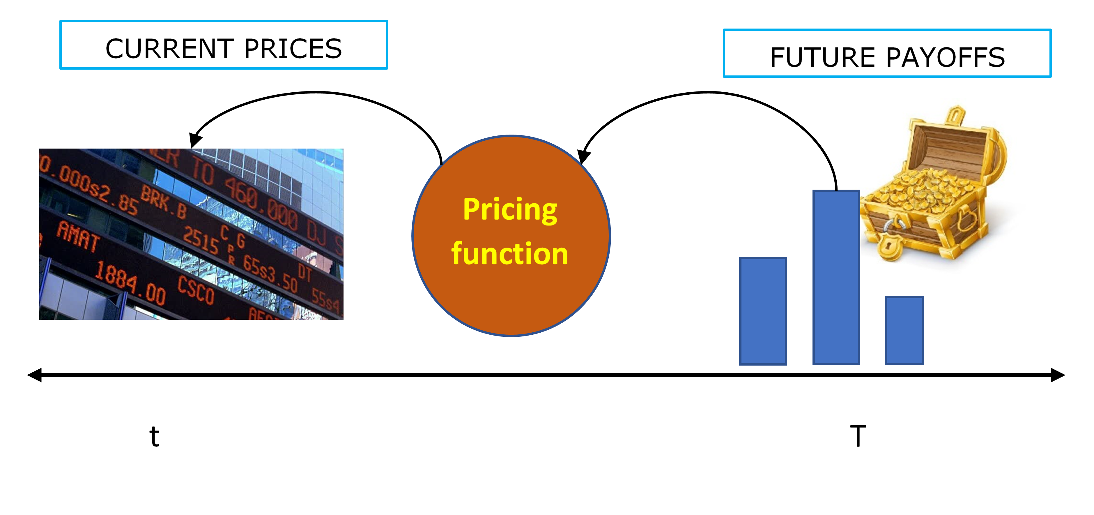
• In a consumption-based asset price model the kernel is linked to the consumer utility function.
• The pricing kernel behaves as if it were a human pricing securities.

Rates of return and prices

For an asset that delivers with certainty a payoff $ \(x_{t+1}\) tomorrow has a price of

\[ p_t = \underbrace{\frac{1}{1+r}}_{\text{pricing kernel}} x_{t+1}. \] with \(r\) the risk-free rate.

• The asset’s price can change because the interest rate does (the pricing kernel) or the future payoff does.

Arbitrage condition under certainty

Under certainty all assets have the same rate of return \(r\).

• Assume that there is a risk-free asset with a net return of \(r=0.05\).
• Consider the following 1-year zero-coupon bonds

Bond	\(p_t\)	Face value
A	956	1000
B	890	1000

• Does the non-arbitrage condition hold?

Arbitrage condition under certainty

Assume that there is a risk-free asset with a net return of \(r=0.05\).

Bond	\(p_t\)	Face value	Net return
A	956	1000	0.046
B	890	1000	0.12

• You would buy bond B and sell bond A. You would make a risk less profit of $ 66.
• Everyone else would do the same and the price of bond B would go up and the price of bond A would go down.

Non-arbitrage condition

With only two periods, a safe bond with return \(r\) and another safe asset with price tomorrow of \(p_2\),

\[ 1+r = \frac{p_2}{p_1} \]

• if \(1+r>p_2/p_1\) then you can make a riskless profit by
  • buying the asset and selling the bond.

EFFICIENT MARKET HYPOTHESIS (EMH)

The efficient market hypothesis states that the price of an asset reflects all available information.

• Suppose that you (and only you) got information that bond A will pay \(\color{blue}{\$150}\) more than expected.
• Assume that there is a risk-free asset with a net return of \(r=0.05\).
• Consider the following 1-year zero-coupon bonds

Bond	\(p_t\)	Face value
A	956	1000+\(\color{blue}{\$150}\)
B	890	1000

• What would you do?

• Buy A and in doing so you change its market price

• \(r^{A}=1.203\) with \(r^{B}=1.124\)

• The result is that the price of bond A would go up reflecting the new information

Fully reflect all available information

Malkiel (1989, p. 127)

“A capital market is said to be efficient if it fully and correctly reveals all available information in determining security prices.
Formally, the market is said to be efficient with respect to some information set, \(\phi\), if security prices would be unaffected by revealing that information to all participants. Moreover, efficiency with respect to an information set, \(\phi\), implies that it is impossible to make economic profits by trading on the basis of \(\phi\).”

\[ R_{i, t+1}= \Theta_{i t} + U_{i, t+1} \]

• \(\Theta_{i t}\) is the equilibrium return on asset \(i\) generated by some economic model,
• \(U_{i, t+1}\) is a fair game with respect to the information set at \(t\), \(\mathbb{E}(U_{i, t+1} | \phi) = 0\)
• Rejection of the equation above implies that the information set at \(t\), \(\phi_{t}\) can be used to trade profitably in the asset, earning higher returns than those captured by the economic model in \(\Theta\).
• The hypothesis refers to both the cross-section and time-series of returns

Weak, semi-strong and strong form

\[ R_{i, t+1}= \Theta_{i t} + U_{i, t+1} \]

• Assessing the efficiency of the market requires a model that generate equilibrium returns \(\Theta_{i,t}\)

• Even when we have such a model what do we include in the information set \(\phi\)?

• Fama (1970)

  • Weak form, \(\phi = \left\{ r_{t-1}, r_{t_2}, \ldots, r_{t-n} \right\}\)
  • Semi-strong form, \(\phi = \left\{ r_{t-1}, r_{t_2}, \ldots, r_{t-n}, d_{t-1}, \pi_{t-1}, \ldots \right\}\)
  • Strong form, \(\phi = \left\{ r_{t-1}, r_{t_2}, \ldots, r_{t-n}, d_{t-1}, \pi_{t-1}, \ldots , \text{private information} \right\}\)

Alternatives to the EMH

Imperfect information processing

• Slugish reaction to information
• Generates short-run continuation of returns following information releases.
• The market may overreact generating reversals.

Persistent mispricing

• Market prices can deviate substantially from efficient levels
• The deviations are hard to arbitrage because they last a long time.
• This generates long-run reversal and predictability based on price levels but may be hard to detect in the short run.

EMH implies unpredictability

• But not the other way around!

“There is no other proposition in economics which has more solid empirical evidence supporting it than the Efficient Markets Hypothesis.”
Michael Jensen (1978)

Jensen’s alpha

Unpredictability does not implies efficiency

“Returns on speculative assets are nearly unforecastable; this fact is the basis of the most important argument in the oral tradition against a role for mass psychology in speculative markets.
One form of this argument claims that because real returns are nearly unforecastable, the real price of stocks is close to the intrinsic value, that is, the present value with constant discount rate of optimally forecasted future real dividends.
This argument… is one of the most remarkable errors in the history of economic thought.”
Robert J. Shiller

cryptocurrencies are alos unforecastable and yet no notion of intrinsinc value

Micro and macro efficiency

Modern markets show considerable micro efficiency (for the reason that the minority who spot aberrations from micro efficiency can make money from those occurrences and, in doing so, they tend to wipe out any persistent inefficiencies).
In no contradiction to the previous sentence, I had hypothesized considerable macro inefficiency, in the sense of long waves in the time series of aggregate indexes of security prices below and above various definitions of fundamental values.
Paul A. Samuelson

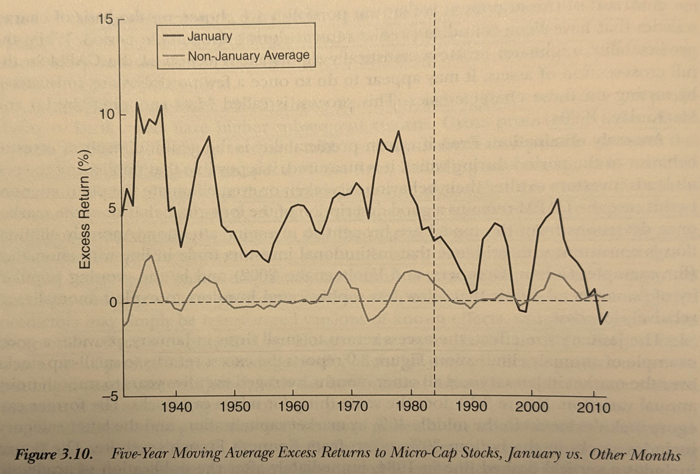
The January effect

• If new information about returns is released the behaviour of markets participants make that this information is quickly incorporated into prices

• This information include scientific articles on asset price models!

• In June 1983, Donald B. Keim published in the Journal of Financial Economics the article “Size-related anomalies and stock return seasonality: Further empirical evidence”

“Evidence is provided that daily abnormal return distributions in January have large means relative to the remaining eleven months, and that the relation between abnormal returns and size is always negative and more pronounced in January than in any other month” (…) ”Further, more than fifty percent of the January premium is attributable to large abnormal returns during the first week of trading in the year, particularly on the first trading day.”

Marc R. Reinganum in the same issue published “The anomalous stock market behavior of small firms in January: Empirical tests for tax-loss selling effects”

The January effect

(2013 Economic Nobel laurates lecture)[https://www.youtube.com/watch?v=WzxZGvrpFu4]

THE CONSUMPTION-BASED ASSET PRICE MODEL

ASSET PRICES AS A UTILITIY MAXIMIZATION PROBLEM

Power utility

With period-utility of the power form, \[ u(c) = \frac{c^{1-\gamma}-1}{1-\gamma} \]

with \(MU(c) = c^{-\gamma}\).

Power utility with \(\gamma =3\)

What the heck does \(\gamma\) do?

• \(\gamma\) controls the curvature of the utility function.
• We know this relates to risk aversion be driving the wedge between \(\mathbb{E}V(\mathcal{L})\) and \(\mathbb{E}[u(\mathcal{L})]\).

Arrow-Pratt measure of risk aversion

• With power utility \(MU(c) = c^{-\gamma} = u^{\prime}(c)\)
• The Arrow-Pratt measure of risk aversion is given by \[ ARA(c) = -\frac{u^{\prime \prime}(c)}{u^{\prime}(c)} = \gamma c^{-1} \]

Demand for an asset with no risk

\[ \max_{I} U(c_1, c_2) = u (c_1)+ \delta u (c_2) \quad \text { subject to} \]

\[ \begin{align} c_1 &=y_1 - p_1 I \\ c_2 &= y_2 + x_2 I \end{align} \]

with \(y_t\) is the income or endowment in period \(t\) and \(x_2\) is the payoff of the asset in period 2.

Substituting into the ojective function we have \[ \max_{I} U(c_1, c_2) = u (y_1 - p_1 I)+ \delta u (y_2 + x_2 I) \] and we only need to find the \(I\) value that maximises this function

Condition for optimum (again)

\[ \max_{I} U(c_1, c_2) = u (y_1 - p_1 I)+ \delta u (y_2 + x_2 I) \]

• We know that we will keep buying the asset until the marginal benefit is equal to the marginal cost of doing so

\[ \begin{align} \frac{\partial U}{\partial I} &= \text{MU}(c_1) (-p_1) + \delta \text{MU}(c_2) x_2 = 0 \\ \underbrace{ p_1 \text{MU}(c_1) }_{\text{Marginal cost}} &= \underbrace{ \delta x_2 \text{MU}(c_2) }_{\text{Marginal benefit}}. \end{align} \]

Marginal cost = marginal benefit

\[ \underbrace{ p_1 \text{MU}(c_1) }_{\text{\textcolor{red}{Marginal cost}}} = \underbrace{ \delta x_2 \text{MU}(c_2) }_{\text{\textcolor{blue}{Marginal benefit}}}. \]

• \(\color{red}{\uparrow I}\) has a marginal cost of
  • \(p_1\) the monetary cost of buying an additional \(I\),
  • the foregone utility of consumption in \(t=1\).
• \(\color{blue}{\uparrow I}\) has a marginal benefit of
  • \(\delta x_2\) the discounted monetary value of the payoff in \(t=2\)
  • the marginal utility of consumption in \(t=2\).

The term on the right is the discounted marginal benefit of buying an additional asset.

The asset price

Solving for the price in \(p_1 \text{MU}(c_1) = \delta x_2 \text{MU}(c_2).\) \[ p_1 = \underbrace{ \delta \frac{ \text{MU}(c_2) }{\text{MU}(c_1)} }_{\text{Discount factor}} x_2. \]

Example with power utility

With period-utility of the power form \(MU(c) = c^{-\gamma}\),

\[ p_1 = \delta \left(\frac{c_{2}^{-\gamma}}{c_1^{-\gamma}}\right) x_{2} = \delta \left(\frac{c_{2}}{c_1}\right)^{-\gamma} x_{2} = \delta \frac{1}{\left(\frac{c_{2}}{c_1}\right)^{\gamma}} x_{2}. \]

The asset price with power utility

\[ p_1 = \delta \frac{1}{\left(\frac{c_{2}}{c_1}\right)^{\gamma}} x_{2}. \]

• \(\uparrow \delta\) means that the consumer is more patient and will pay more for the asset.

the consumer values more consumption in period 2

• \(\uparrow x_2\) a higher future payoff increases the price because the asset delivers a higher consumption in \(t=2\).

Consumption smoothing and the safe asset price

\[ p_1 = \underbrace{ \delta \frac{ \text{MU}(c_2) }{\text{MU}(c_1)} }_{\text{Discount factor}} x_2. \]

• Let consumption growth be \(c_2/c_1\)
• Consumption growth reduces the price of the asset
  • because the consumer has lower needs to transfer more consumption from \(t=1\) to \(t=2\).
  • Desire to smooth consumption over time.
  • this is embedded in the convexity of the indifference curves

Consumption smoothing and the safe asset price

• With power utility \[ p_1 = \delta \frac{1}{\left(\frac{c_{2}}{c_1}\right)^{\gamma}} x_{2}. \]

  • \(\uparrow \frac{c_2}{c_1}\) reduces the asset price.

The risk-free interest rate with certain consumption

Assume a bond that pays \(x_2 = 1\), then \[ 1+r \equiv \frac{p_2}{p_1} = \frac{x_2}{p_1} = \frac{1}{p_1} = \frac{1}{\delta \frac{ \text{MU}(c_2) }{\text{MU}(c_1)}} \]

• With power utility \(MU(c) = c^{-\gamma}\) \[ 1+r = \frac{1}{ \delta \left( \frac{ c_2 }{ c_1} \right)^{^{-\gamma}}} = \frac{1}{\delta} \left(\frac{ c_2 }{ c_1} \right)^{\gamma} \]

The risk-free rate with power utility

\[ 1+r = \frac{1}{\delta} \left(\frac{ c_2 }{ c_1} \right)^{\gamma} \]

• The risk-free is low when people are patient
• \(\color{blue}{\uparrow} \delta\), \(\downarrow 1+r\)

a higher subjective discount factor \(\delta\) implies people saves more because they value more future consumption thus the interest rate is lower.

The risk-free rate and consumption growth

• With power utility \(MU(c) = c^{-\gamma}\) \[ 1+r = \frac{1}{\delta} \left(\frac{ c_2 }{ c_1} \right)^{\gamma} \]

• The risk-free rate is high when consumption growth is high

• \(\color{blue}{\uparrow} c_2/c_1\), \(\uparrow 1+r\).

• Alternatively, if \(1+r\) is high, the consumer consumes less today and saves more for tomorrow thus \(\uparrow c_2/c_1\).

Sensitivity to consumption growth

• With power utility \(MU(c) = c^{-\gamma}\)

\[ 1+r = \frac{1}{\delta} \left(\frac{ c_2 }{ c_1} \right)^{\gamma} \]

• The risk-free rate is more sensitive to consumption growth when \(\gamma\) is larger
• With \(\gamma = 1\)
  • \(c_2/c_1 = 1.02\), \(1+r\) is \(1.041\)
  • \(c_2/c_1 = 1.04\), \(1+r\) is \(1.061\). \(\color{blue}\Delta (1+r) = 0.02\).
• With \(\gamma = 2\)
  • \(c_2/c_1 = 1.02\), \(1+r\) is 1.062
  • \(c_2/c_1 = 1.04\), \(1+r\) is 1.104. \(\color{blue}\Delta (1+r) = 0.042\).

INTRODUCING RISK

• Now the asset has a risky payoff \(x_2\) and the consumer has an stochastic endowment in period 2, \(y_2\)
• The consumer maximises expected utility.

\[ \max_{I} U(c_1, c_2) = u (c_1)+ \delta \mathbb{E} u (c_2) \quad \text { subject to} \]

\[ \begin{align} c_1 &=y_1 - p_1 I \\ c_2 &= \mathbb{E}_1(\tilde{y_2}) + \mathbb{E}_1(\tilde{x_2}) I \end{align} \]

with condition for optimum \[ p_1 MU(c_1) = \delta \color{blue}{\mathbb{E}_1} [ x_2 MU(c_2) ] \]

The stochastic discount factor (SDF)

\[ p_1 MU(c_1) = \delta \mathbb{E}_1 [ x_2 MU(c_2) ] \] solving for the price

\[ \begin{align} p_1 &= \frac{\delta \mathbb{E}_1 [ x_2 MU(c_2) ]}{ MU(c_1)} \\ p_1 &= \mathbb{E}_1 \left[ \delta \frac{ MU(c_2) }{ MU(c_1)} x_2 \right] \\ \end{align} \]

• Now let \(m_2 \equiv \delta \frac{ MU(c_2) }{ MU(c_1)}\) we have \[ p_1 = \mathbb{E}_1 \left( m_2 x_2 \right) \]
• \(m_2\) is the stochastic discount factor (SDF) at time \(t=2\).
• It is a random variable that is used to discount future payoffs to their present value.
• \(m_2\) and \(x_2\) are random variables

What about returns?

Let \(R_{i} \equiv \frac{x_{i,t}}{p_1}\) be the gross return on asset \(i\) between \(t=1\) and \(t=2\).

\[ 1 = \mathbb{E}\left(m_2 \frac{x_2}{p_1} \right) \]

\[ 1 = \mathbb{E}\left(m_2 R_i \right) \]

• This applies to every asset \(i\)
• The expected risk-adjusted gross return for every asset is 1.
  • This is the non-arbitrage condition

The risk-free rate in SDF form

• The return on the risk-free asset is known at \(t=1\), \[ 1+r = \frac{p_2}{p_1} = \frac{x_2}{p_1} = \frac{1}{p_1} \] where \(p_2\) is the price of the risk-free asset at \(t=2\).

Ergo, \[ p_1 = \frac{1}{1+r} 1 \]

• The SDF prices any asset including the risk-free asset.
• Thus we can write \[ p_1 = \mathbb{E}_1 \left( m_2 x_2 \right) = \mathbb{E}_1 \left( m_2 \right) 1 \]

The risk-free rate in SDF form

\[ p_1 = \mathbb{E}_1 \left( m_2 x_2 \right) = \mathbb{E}_1 \left( m_2 \right) 1 \]

• The mean of the SDF is the price of the risk-free asset
• The inverse of the mean of the SDF is the risk-free rate \[ 1+r = \frac{1}{\mathbb{E}_{t=1} \left( m_{t=2} \right)} \]

The risk-free interest rate with risky consumption

\[ 1+r = \frac{1}{\mathbb{E}_{t=1} \left( m_{t=2} \right)} \]

• Recall \(m_2 \equiv \delta \frac{ MU(c_2) }{ MU(c_1)}\)

• With power utility \(MU(c) = c^{-\gamma}\) \[ 1+r = \frac{1}{ \delta \,\, }\mathbb{E}_{t=1} \left( \frac{ c_2 }{ c_1} \right)^{\gamma} \]

• The risk-free depends on consumption growth \(c_2/c_1\)

  • Let \(\color{blue}{\Delta \ln c_2} \equiv \ln(c_2) - \ln(c_1)\)
  • Note that \(\frac{c_2}{c_1} = \ln(c_2) - \ln(c_1) = \color{blue}{\Delta \ln c_2}\)

The risk-free interest rate with risky consumption

\[ 1+r = \frac{1}{ \delta \,\, }\mathbb{E}_{t=1} \left( \frac{ c_2 }{ c_1} \right)^{\gamma} \]

• Recall ¡risk-free only means default risk!
• Let consumption growth be lognormally distributed
• Assume a discount factor \(\delta = e^{-\beta}\), a continuous-time discount factor with \(\beta\) the discount rate
• It can be proved that \[ \ln (1+r) = \beta + \color{red}{\gamma} \mathbb{E}_1 (\color{blue}{\Delta \ln c_2}) - \frac{1}{2} \color{red}{\gamma}^2 \sigma_t^2 (\color{blue}{\Delta \ln c_2}) \] where \(\sigma_t^2 (\color{blue}{\Delta \ln c_2})\) is the expected variance on consumption growth.

The risk-free rate with risky consumption

\[ \ln (1+r) = \beta + \gamma \mathbb{E}_1 (\Delta \ln c_2) - \frac{1}{2} \gamma^2 \sigma_t^2 (\Delta \ln c_2) \]

• the interest rate is higher when people are more impatient (a higher discount rate \(\beta\))
• the interest rate is higher when people are more risk averse, a higher \(\gamma\)
• the interest rate is higher when expected consumption growth is higher
• the interest rate is lower when the volatility on consumption growth is higher (precautionary savings)
  • when consumption is more volatile people with this utility function are more worried about drops in consumption that what they are pleased with increments in consumption, thus they save more driving down the interest rate

The risk premium in SDF form

• Every asset \(i\) is priced by the same \(m_2\).
• The asset specific risk premium is captured by the covariance between the asset payoff and the SDF.
• The covariance between an specific asset \(i\) and the SDF determines asset-specific corrections

\[ p_{i,1} = \mathbb{E}\left(\color{blue}{m_2} x_{i,2} \right) = \mathbb{E}(\color{blue}{m_2}) \mathbb{E}(x_{i,2}) + \operatorname{\mathbb{C}ov}(\color{blue}{m_2}, x_{i,2}) \] with \(\mathbb{E}(\color{blue}{m_2}) = 1/(1+r)\) \[ p_{i,1} = \frac{\mathbb{E}(x_{i,2})}{1+r} + \underbrace{\operatorname{\mathbb{C}ov}(\color{blue}{m_2}, x_{i,2})}_{\text{risk adjustment}} \]

• The price of any risky asset is the discounted value of the expected payoff of a risk-neutral consumer plus
• A risk adjustment or risk premium component.

Consumption and the risk premium

• Assets that deliver higher payoffs when consumption is low have greater prices.
• Assets that deliver higher payoffs when consumption is high have lower prices.

\[ p_{i,1} = \frac{\mathbb{E}(x_{i,2})}{1+r} + \frac{\operatorname{\mathbb{C}ov} \left[ \delta MU(c_2), x_{i,2}) \right]}{MU(c_1)} \]

• \(\color{blue}{\uparrow} c\), \(\color{red}{\downarrow} MU(c)\)

• if \(\color{blue}{\uparrow} x_{i,2}\) when \(\color{blue}{\uparrow} c_2\) then

• \(\color{red}{\downarrow} MU(c_2)\) when \(\color{blue}{\uparrow} x_{i,2}\) and the \(\operatorname{\mathbb{C}ov}<0\)

• \(\color{red}{\downarrow} p_{i,1}\)

• When the asset payoffs are positively correlated with consumption the investor values less this asset because it delivers when you don’t need it

  • The asset is not a good hedge against drops in consumption

Volatility of consumption and the risk premium

• The risk premium is the covariance between the SDF and the asset payoff, not the variance of the asset payoff
• The investor cares about volatility of consumption, not the volatility of the asset payoff itself
• To see this suppose what happens if the investor \(\color{blue}{\uparrow} I\), how much does \(\sigma^2(c)\) change?

\[ \sigma^2(c + Ix) = \sigma^2(c) + I^2 \sigma^2(x) + 2I \operatorname{\mathbb{C}ov}(c, x) \]

• For small changes in \(I\), say \(\Delta I = 0.10\), the volatility of consumption is primarily determined by the last term rather than by \(I^2 \sigma^2(x)\)

KEY IDEAS in KEY EQUATIONS

With certain payoffs

The price of the asset

\[ p_1 = \underbrace{ \delta \frac{ \text{MU}(c_2) }{\text{MU}(c_1)} }_{\text{Discount factor}} x_2. \]

With power utility:

\[ p_1 = \delta \frac{1}{\left(\frac{c_{2}}{c_1}\right)^{\gamma}} x_{2}. \]

Real interest rate with certain payoff and consumption growth

\[ 1+r = \frac{1}{ \delta} \left( \frac{ c_2 }{ c_1} \right)^{^{\gamma}} \]

With uncertain payoffs

The price of the asset in SDF from

\[ p_1 = \mathbb{E}_1 \left( m_2 x_2 \right) \]

Real interest rate with risky payoff

\[ 1+r = \frac{1}{\mathbb{E}_{t=1} \left( m_{t=2} \right)} \]

Risk premium is covariance with the SDF. With power utility

\[ p_{i,1} = \frac{\mathbb{E}(x_{i,2})}{1+r} + \frac{\operatorname{\mathbb{C}ov} \left[ \delta MU(c_2), x_{i,2}) \right]}{MU(c_1)} \]